
Halbach Array Magnetic Field Mapping & Acceptance Testing: 3D Hall Scanning, Helmholtz Vector Deviation, and FAT Verification for Custom Assemblies
Plan Halbach array magnetic field mapping: compare Hall scans, Helmholtz vector checks and FAT records. Use the checklist to prepare your inspection RFQ.
Halbach array magnetic field mapping turns a promise of “magnetic inspection” into measurable acceptance criteria. For procurement teams and magnetic-system engineers, the practical approach is to check individual magnet vectors before bonding, map the assembled working field at a defined location, and agree a Factory Acceptance Testing (FAT) data package before placing the order. A single peak Gauss reading cannot establish field uniformity, harmonic content, or leakage across an entire assembly.
Published and technically reviewed: November 11, 2026. This guide covers custom permanent-magnet Halbach tracks, rotors, and bore assemblies for global sourcing. It is an inspection-planning framework, with explicitly illustrative calculations, rather than measured factory results or an application approval. Numerical acceptance limits must come from the system requirements, simulation, measurement uncertainty, and an agreed drawing revision. Medical, aerospace, and high-speed rotor qualification require additional application-specific validation.
If a purchase order is being prepared, send the drawing and proposed inspection requirements for review. Include the working gap, field component, temperature, and required deliverables so that suppliers quote the same inspection scope.
1. The "Black Box" Problem in Halbach Metrology
Two arrays can meet the same dimensional drawing yet produce different working fields. Segment polarity, magnetization direction, material variation, bond-line thickness, and the assembly's thermal history all affect the result. Mechanical inspection remains necessary; magnetic inspection adds evidence about the assembled function.
A linear sequence using four segments per magnetic wavelength rotates the intended magnetization by 90 degrees at each segment. Eight segments per wavelength would use 45-degree steps. A wavelength includes a complete repeating sequence, rather than a single north or south pole. Curved arrays require a geometry-specific vector convention; do not transfer the linear sequence directly to every cylindrical design.
Potential problems include a reversed segment, angular misalignment relative to its mounting datum, excessive adhesive gaps, and irreversible demagnetization during curing. Their effects depend on geometry and operating point. A local field dip alone does not prove which defect occurred.
Why an Uncontrolled Single-Point Gauss Check Is Insufficient
A calibrated gaussmeter can support acceptance when its probe is properly fixtured and the specified measurement is sufficient for the application. The main weakness of an unfixtured reading is the uncertain sensor position and orientation.
For an ideal, infinitely extended planar Halbach fundamental at a fixed phase, field amplitude decays with lift-off approximately as:
This is a sensitivity model, not a universal field solution for finite tracks, end regions, or cylindrical bores. For an illustrative wavelength of 20 mm, increasing lift-off by 0.10 mm gives a field reduction of . At a 6 mm wavelength, the same displacement gives 9.94%. Specify distance to the active sensing element, including its offset behind the probe tip, rather than simply pressing the probe housing against the magnet.
Probe tilt also mixes field components. A single-axis sensor tilted toward the longitudinal direction measures approximately . Correcting only the cosine term is inadequate when the orthogonal component is appreciable. Finally, a Hall sensor averages over its finite active area. Lake Shore's Hall probe selection guide explains why active area and tip-to-sensor distance matter in steep gradients.
2. Stage 1: Pre-Assembly Vector Screening via Helmholtz Coils
Pre-assembly screening identifies unsuitable segments while they can still be replaced without disturbing a bonded array. IEC 60404-14:2002 describes open-circuit dipole-moment measurement using detection coils and withdrawal or rotation. It provides a measurement-method reference; it does not prescribe a universal Halbach angle tolerance, mandatory three-axis apparatus, or 100% inspection requirement.
The Helmholtz Moment Equation
A Helmholtz pair consists of two coaxial circular coils whose separation equals their radius. A calibrated detection-coil system and integrating fluxmeter measure the change in flux linkage as a specimen is withdrawn or rotated. Define the instrument's effective sensitivity for the actual measurement motion as:
Here is the moment component in A·m² and includes the coil calibration and withdrawal or rotation convention. A 180-degree reversal changes the signed component from positive to negative; its factor of two must be included in the reduction. Specimen size, placement, integration drift, background subtraction, and calibration validity belong in the procedure.
Use the symbol for dipole moment; magnetization is moment per unit volume and has different units. Measuring moment alone does not establish alloy chemistry, coercivity, or resistance to thermal demagnetization. For material-property testing and demagnetization curves, IEC 60404-5:2015 is the relevant companion method reference.
Resolving True 3D Magnetization Angle Deviation
Three orthogonal coil channels, or repeat measurements with controlled specimen reorientation, can resolve . Record how the fixture's axes align with the segment's mechanical datums. For a segment intended to point along positive Z:
This angle ranges from zero to 180 degrees and therefore distinguishes a reversed magnet. A simple one-argument arctangent loses that distinction. For another intended direction, calculate the angle between the measured vector and the drawing's nominal unit vector. Retain signed transverse components as well as the unsigned angular deviation. Treat a moment at or below measurement resolution as indeterminate rather than assigning a valid angle.
Magnetization Angle Limits and Block Sorting
Angle limits are design inputs. For example, a project might evaluate a 1.5-degree maximum deviation and tighten it after a tolerance study. That number is an illustrative screening choice, not a motor, NMR, or semiconductor industry standard. Check that fixture alignment and measurement uncertainty can resolve the proposed limit before paying for tighter sorting.
Store each segment's identity, moment vector, test temperature, and final assembly position. A simulation-based sorting plan can compare candidate arrangements, but placing opposite signed tilts across a rotor does not automatically cancel all unwanted harmonics. Verify the final assembly after bonding; segment screening cannot detect later movement, cure damage, or installation errors.
3. Stage 2: Automated Multi-Axis 3D Hall Probe Field Mapping
Post-assembly mapping measures the field where the application uses it. “3-axis” describes the measured vector components; “3D mapping” describes spatial coverage. A three-axis probe following one circular track does not create a full volumetric map. State both the trajectory and the acquired components in the RFQ.
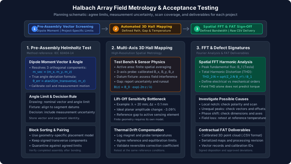
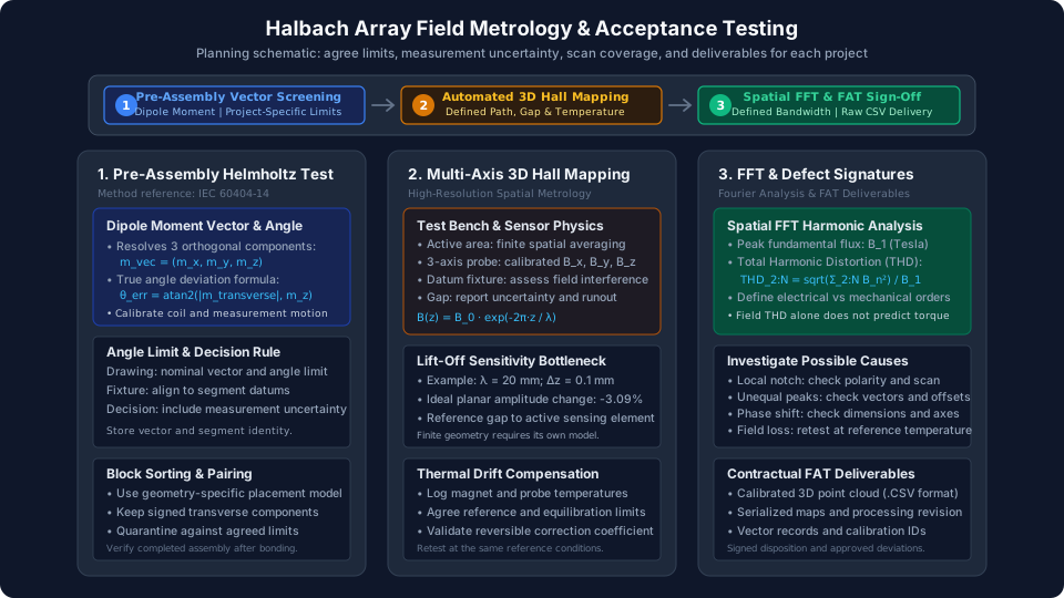
Figure 1. Inspection-planning schematic, not a measured field map or proof of installed factory equipment. Each limit and instrument capability must be agreed for the project.
Test Bench Architecture and Coordinate Systems
Choose a fixture that references the assembly's mounting datums and keeps interfering ferromagnetic hardware away from the mapped region. Assess nearby structures and background fields rather than assuming that a granite base alone removes interference. Stage encoder resolution is not the same as absolute probe-position accuracy or total field-measurement uncertainty.
- Cartesian scanning: A planar track can be scanned on an X/Y raster at specified Z planes. Include both the active region and any end zones relevant to operation.
- Cylindrical scanning: A radial-field rotor can be rotated relative to a fixed probe at defined radii and axial stations. Measure runout and transform laboratory components into radial, tangential, and axial components.
- Bore scanning: A cylinder can be mapped along registered axial, circular, or helical paths. Define the useful volume and ensure that the trajectory supports the required uniformity metric.
For an axial-flux disc, a face scan at defined axial gaps may be more appropriate than an external cylindrical scan. NMR or MRI homogeneity requirements may also demand dedicated high-resolution methods beyond the Hall system's demonstrated capability.
Sensor Physics, Temperature, and Uncertainty
Select probe range, active area, noise, bandwidth, and spatial registration together. Smaller active areas reduce averaging but do not eliminate it. Three-axis probes may have sensing elements at different locations; in a strong gradient, their readings may not represent one coincident point. Request element offsets, calibration range, cross-axis characterization, and the transformation used to report assembly coordinates. A zero-field check detects offsets; it cannot establish scale factors or axis orthogonality.
Record actual magnet temperature after equilibration, as well as probe and ambient conditions. If temperature normalization is used, document the validated reversible coefficient, reference temperature, and applicable interval. Do not use a generic remanence coefficient to correct irreversible loss or to infer coercivity. Compare pre-soak and post-soak scans at the same equilibrated reference temperature when assessing irreversible change.
The uncertainty budget should include calibration, sensor offset, position, runout, angular alignment, finite-area response, temperature, and repeatability. For the ideal 20 mm wavelength example, a 0.005 mm lift-off contribution alone corresponds to about 0.157% field variation. Micrometre stage repeatability therefore cannot, by itself, establish a complete magnetic accuracy claim.
4. Mathematical Processing: Spatial FFT Harmonic Decomposition & THD
Spatial Fourier analysis converts a periodic field track into amplitude and phase metrics. It is useful for repeating motor or track fields; bore homogeneity and finite end fields may require different metrics. Define the sampled component and path before comparing spectra.
The Spatial Fourier Series
For a periodic linear field component, including a possible DC offset:
On a rotor, distinguish mechanical orders per revolution from electrical harmonics relative to the intended pole-pair order. Define as the intended electrical fundamental, not automatically the first FFT bin of a mechanical revolution. Use a consistent peak or RMS amplitude convention throughout.
Segmentation, finite geometry, and assembly errors can all create harmonics. Even-order terms may indicate lost half-wave symmetry, but they do not uniquely diagnose an inverted block. A small field THD also does not guarantee low torque ripple: winding distribution, current control, slotting, and mechanical dynamics affect system performance.
Total Harmonic Distortion and a Reproducible Example
A measured spectrum has a finite analyzed bandwidth. Report the highest retained order and use:
Illustrative calculation, not test data: Let T, T, and T, with all other included harmonic amplitudes set to zero. Then . This would satisfy an illustrative 2.5% THD limit only under the agreed bandwidth and decision rule. Real omitted harmonics and uncertainty can change the verdict.
For analysis through order 15, uniformly sampling 64 positions per electrical wavelength is an example acquisition choice exceeding the Nyquist minimum of more than 30. It is not sufficient evidence that sharp local defects have been resolved. Specify spatial filtering, scan speed, sensor response, and any denser coverage needed for localized anomalies. Avoid duplicating the start point at the end of a periodic record. Use an integer number of periods or document windowing and amplitude corrections to control spectral leakage.
Keep raw coordinates and calibrated field components alongside the spectrum. A supplier's processed THD figure is difficult to reproduce without those inputs and the processing revision. Before finalizing an inspection budget, compare the proposed field test with the assembly quote scope.
5. Application-Specific Acceptance Planning Matrix
The following matrix identifies requirements to close before issuing an order. It deliberately avoids universal numerical limits: an acceptable field at one air gap, volume, or temperature cannot qualify a different application. The buyer's system engineer owns the limits; the supplier must demonstrate that its measurement method can resolve them.
| Application | Mapping location | Primary acceptance metric | Additional check | Requirement to freeze before FAT |
|---|---|---|---|---|
| Semiconductor positioning track | Specified X/Y area at operating Z planes | Fundamental amplitude and spatial uniformity | End effects and transverse components | Active travel region, force-error budget, datum and temperature |
| Radial-flux motor rotor | Cylindrical tracks at agreed radii and axial stations | Radial fundamental, phase and specified harmonic orders | Runout and axial variation | Pole-pair convention, radius, loaded-system validation boundary |
| Axial-flux motor disc | Face raster or circular paths at axial working gaps | Axial field amplitude and pole consistency | Inner/outer radius and edge effects | Radial coverage, face datum and angular registration |
| NMR or MRI bore | Defined useful bore volume | Field uniformity relative to a named reference field | Temperature stability and shimming state | Volume, ppm definition and demonstrated instrument resolution |
| Magnetic gear | Working cylindrical gaps for the relevant member | Intended multipole amplitude and spatial phase | Modulator influence and leakage | Assembled configuration and link to torque testing |
| Magnetic bearing | Defined radial/axial locations | Agreed field components and symmetry | Eccentricity sensitivity | Relation to force/stiffness tests and rotor qualification |
| Maglev or linear drive track | Defined travel path at operating gaps | Field amplitude, pitch and repeatability | Track joints and end zones | Gap range, joint inclusion and scan speed |
For a uniformity requirement, define the arithmetic. “Peak-to-peak divided by mean” and “maximum absolute deviation from reference” are different metrics. For a signed periodic component with a near-zero mean, normalizing by the mean is unsuitable; use an agreed fundamental amplitude, pole peak, or other nonzero reference.
6. Defect Signatures: Investigating Assembly Failures from Field Scans
Use maps to guide investigation, then corroborate suspected causes with segment records, dimensions, temperature history, and a registered remeasurement. Similar field patterns can arise from different faults or from the measurement setup itself.
- Localized notch or field collapse: Check segment polarity and orientation records, but first exclude a position jump or probe saturation. Quarantine the affected assembly pending confirmation.
- Unequal positive and negative peaks: Investigate magnetization vectors, segment positions, sensor offsets, and coordinate alignment. Harmonic amplitude alone cannot assign responsibility to the material supplier.
- Local phase displacement near a joint: Compare bond-line and carrier dimensions with the drawing. A shifted segment and a measurement-coordinate error can look similar in the field trace.
- Reduced amplitude after thermal exposure: Repeat the map after returning to the original reference temperature. Review operating point, grade-specific demagnetization curves, and cure history before attributing the difference to irreversible loss.
A proposed change to magnet grade, adhesive, or assembly tooling should return through engineering review and a defined requalification plan. It cannot be approved solely by matching a visual defect pattern.
7. The 10-Point Contractual Factory Acceptance Testing (FAT) Checklist
Use this checklist to agree a project-specific inspection annex with the supplier. It defines the evidence required for release and the handling of uncertain or nonconforming results.
- 1. Segment traceability: Define whether every segment or a specified sample receives vector screening. Record lot/segment identity, moment units, nominal direction, angle limit, fixture alignment, and the applicable method revision.
- 2. Material evidence: Specify grade and required material-property reports separately from assembled field tests. Record the basis for any temperature coefficient used in correction.
- 3. Mechanical datums: Define the coordinate origin, axis directions, angular zero, field sign convention, and inspection drawing revision.
- 4. Working gap: Specify distance from an identified assembly surface to the active sensing element. Include coatings, retention sleeves, probe offsets, and allowed position uncertainty.
- 5. Temperature: Agree reference temperature, equilibration criterion, allowed variation, sensor placement, and whether validated normalization is permitted.
- 6. Coverage and acquisition: Freeze trajectories, regions, grid pitch, scan speed, field range, repeated measurements, and treatment of edges and joints.
- 7. Processing and field limits: Define amplitude convention, fundamental order, retained harmonic orders, THD bandwidth, filtering, and limits for each required component or uniformity metric.
- 8. Measurement decision rule: Require the uncertainty statement and agree how results near a limit are handled. Define pass, fail, and hold-for-review conditions before testing begins.
- 9. Conditioning and retest: Specify any thermal, vibration, or rotational conditioning appropriate to the assembly and its containment. Repeat registered scans at the same reference conditions; field mapping alone does not qualify retention, balance, or overspeed safety.
- 10. FAT package and release: Request serialized raw CSV/JSON data, units, coordinate definitions, calibration identifiers, environmental logs, field plots, processing revision, and signed disposition. Record approved deviations and responsibility for rework or retest.
For example, a buyer might agree that an upper field limit passes only when the measured value plus expanded uncertainty is no greater than . A reading whose uncertainty interval overlaps the limit would then be held for review. This is an illustrative guard-band rule; agree the actual rule and uncertainty coverage with both parties, including how it applies to derived metrics such as THD.
8. Frequently Asked Questions (FAQ)
Can we use a calibrated handheld Gauss meter for incoming receiving inspection?
Yes, if the defined inspection can be met with a controlled fixture, suitable probe, repeatable coordinates, and demonstrated uncertainty. A freely positioned spot reading is useful for polarity screening but does not establish a full field map. Supplier and buyer should use equivalent sensing positions and methods when comparing results.
If an assembled Halbach array fails due to an inverted segment, can the factory repair it?
Repairability depends on the carrier, adhesive, retention method, and access. Removing a bonded segment can damage neighboring magnets or disturb other bond lines. Request a documented rework proposal and repeat the affected inspections after repair. Pre-assembly screening reduces avoidable rework, but it does not replace orientation controls during assembly.
Why does our 3D Hall scan show lower peak flux than our simulation?
First align the simulation and measurement definitions: coordinates, active gap, temperature, sampled component, sensor area, and actual assembled geometry. Compare measured material properties and bond lines with model assumptions. A point-value FEA output is not directly equivalent to a finite-area Hall reading. Treat discrepancies as a reconciliation task before deciding that either the material or the scanner is defective.
What is the advantage of cylindrical scanning for motor rotors?
For radial-field rotors, rotation at defined radii makes circumferential coverage practical. Accuracy still depends on axis registration, runout, sensor alignment, and coordinate transformation. It does not automatically eliminate tilt error, and an axial-flux rotor may require a face scan instead.
How does magnet coating thickness impact magnetic field measurement?
Coating thickness changes the distance between the magnetic substrate and the sensing element, so the drawing must identify the gap reference surface. Do not assume every coating is magnetically inert: nickel-containing plating can also affect the local field. Include the actual coating stack in a model when its influence matters to the tolerance, and record whether the acceptance datum is the substrate, coating, or outer sleeve.
Is 100% 3D Hall mapping necessary for volume production?
The inspection plan depends on failure severity, defect mechanisms, process stability, and the ability of a faster screen to detect relevant failures. One possible plan combines qualification maps, a validated production screening path, and periodic full maps. Critical assemblies may justify full mapping on every unit. Agree lot definition, sampling rules, escalation triggers, and disposition of failed lots; an AQL number alone is not an inspection plan or a guarantee of every unit's performance.
9. Securing Metrology-Driven Halbach Sourcing
A useful magnetic acceptance specification connects the system's working field to a reproducible measurement. Segment vectors support assembly control; Hall maps verify the finished field; processing definitions and uncertainty make the FAT verdict interpretable. These checks reduce ambiguity while leaving application performance, mechanical integrity, and regulatory qualification to their respective validation processes.
Review our engineering support overview and quality and assembly capabilities, or use the custom Halbach supplier qualification guide to prepare a comparable RFQ. Ask each candidate supplier to confirm available instruments, calibration coverage, achievable uncertainty, inspection time, and sample report format for your exact geometry.
Contact Halbach Magnet with your drawing and draft FAT checklist to discuss the inspection scope. Include the assembly revision, operating gap and temperature range, target field metrics, order quantity, and requested raw-data format. Confirm feasibility and deliverables in the quotation before treating them as production commitments.
Sources & References
Sources checked November 11, 2026. These support the stated measurement principles and method scopes; they do not establish the illustrative acceptance limits or certify any supplier's equipment.
- IEC 60404-14:2002 — Dipole moment by withdrawal or rotation. Official IEC catalogue scope for open-circuit detection-coil measurements. Consult the full standard when specifying compliance.
- IEC 60404-5:2015 — Permanent magnet material measurement methods. Official IEC catalogue scope for material magnetic properties and demagnetization/recoil curves; distinct from an assembled-array field map.
- Lake Shore Cryotronics — Hall Probe Selection Guide. Manufacturer guidance on probe orientation, active-area averaging, gradients, range, and sensing-element position.
Author

Categories
More Posts

Halbach Array Supply Chain Traceability: Preparing for EU CRMA & CEN/TS 18263:2026
Prepare Halbach magnet sourcing for EU CRMA and CEN/TS 18263:2026 with supplier data fields, recycling risks, RFQ checklist, and contact review steps.

Halbach Array Rotor Retention Sleeves: Carbon Fiber vs. Titanium vs. Inconel
Compare Halbach rotor retention sleeves for high-speed motors: CFRP, titanium, and Inconel trade-offs for eddy losses, thermal limits, and RFQs.
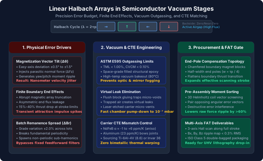
Linear Halbach Arrays for Vacuum Wafer Stages: Mitigating Force Ripple, Boundary End Effects, and CTE Mismatch in Precision Motion Systems
Specify linear Halbach arrays for vacuum wafer stages: mitigate force ripple, boundary end effects, ASTM E595 outgassing, and CTE carrier mismatch in your RFQ.