
Circular Halbach Array

A circular Halbach array rotates magnetization around a ring to concentrate its field. Estimate an ideal bore or external field and magnet mass, then review the design limits below.

2D field & mass calculator

1.197 T2D target fundamental at r = 0 mmInfinite-length reference. Finite-length field and THD require 3D FEA / measurement.

0.1–10,000; bore ID = 2Ri

0.1–10,000; must exceed Ri

0.1–10,000; affects mass only

Bore: 0–Ri; external: Ro–100,000

20–150; N52 reference limited to 60

0–150,000; 0 = static; not a safe limit

At least as many sectors as poles.

Catalog values; confirm supplier curves.

Request engineering review

All inputs required. Dimensional ranges are software limits. No temperature or speed entry constitutes operating approval. Read assumptions and equations.

Fundamental retained kM
0.97450
Full annulus mass
1.178 kg
Remanence at temperature
1.4500 T
L / outer diameter
0.714
Surface speed
0.00 m/s
Inertial scale ρv²
0.00 MPa

Mass excludes glue, sleeve and gaps. ρv² is a screening scale, not actual assembly stress or an allowable limit.

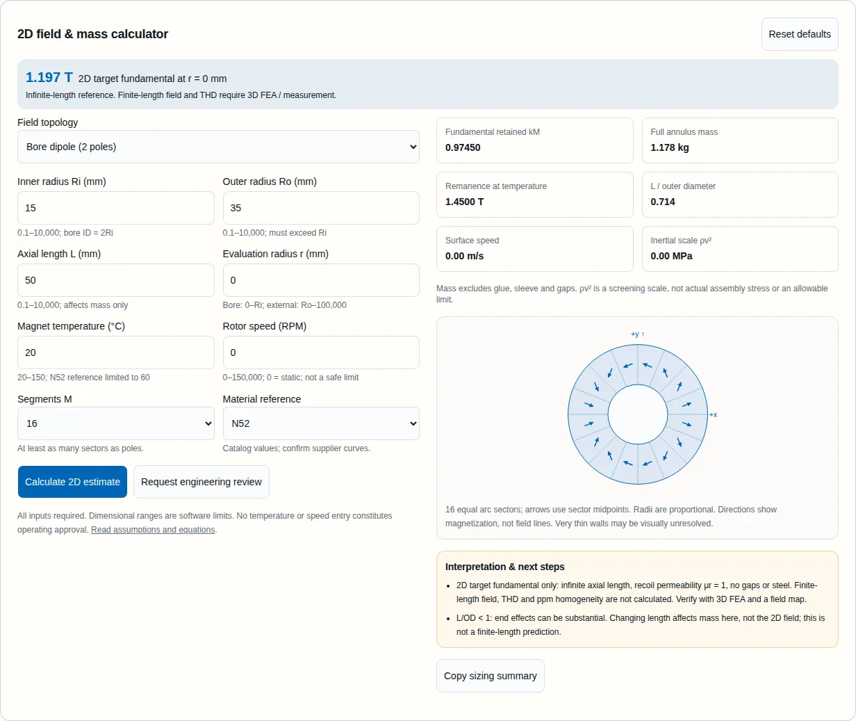
Magnetization directions at sector midpoints; Cartesian angles counterclockwise from +x+y ↑+x
16 equal arc sectors; arrows use sector midpoints. Radii are proportional. Directions show magnetization, not field lines. Very thin walls may be visually unresolved.

Interpretation & next steps

  • 2D target fundamental only: infinite axial length, recoil permeability μr = 1, no gaps or steel. Finite-length field, THD and ppm homogeneity are not calculated. Verify with 3D FEA and a field map.
  • L/OD < 1: end effects can be substantial. Changing length affects mass here, not the 2D field; this is not a finite-length prediction.

1. What the result can help you decide

By Halbach Magnet. First recorded: . Method and source review: . This is a preliminary sizing guide; the examples are calculations, not customer test records.

  • Choose the working region first. An internal dipole targets a bore field; an external multipole targets the outside air gap. A bore formula cannot predict a stator-loaded motor field.[1]
  • Use segmentation to compare fundamental amplitude. A 16-sector dipole retains 97.45% of its continuous reference amplitude. That number does not establish field purity, torque ripple or homogeneity.[2]
  • Length and uniformity need a separate check. The 2D calculation omits end effects. A short ring and a long cylinder with the same radii can have the same displayed 2D field and different measured maps.[5]
  • Select materials against temperature and reverse field. Catalog remanence is a reference input. Obtain supplier B–H curves and verify irreversible loss, rather than treating a grade temperature entry as a safe limit.[3][4]

2. Bore field or external rotor?

Ideal target-field behavior; signed p follows Bjørk et al. [1].
TopologySigned p / direction lawField behaviorDecision
Internal dipole+1; ψ = 2θUniform transverse field in ideal 2D boreStart here for a static uniform-field region
Internal quadrupole+2; ψ = 3θAmplitude proportional to r; zero on axisSpecify gradient and integrated field
Internal hexapole+3; ψ = 4θAmplitude proportional to r²Specify the nonlinear working region
External 8-pole rotor−4; ψ = −3θTarget amplitude proportional to r⁻⁵ outside RoBudget sleeve + gap before comparing flux

Bore dipole (2 poles)

Magnetization directions at sector midpoints; Cartesian angles counterclockwise from +x+y ↑+x
16 equal arc sectors; arrows use sector midpoints. Radii are proportional. Directions show magnetization, not field lines. Very thin walls may be visually unresolved.

Bore quadrupole (4 poles)

Magnetization directions at sector midpoints; Cartesian angles counterclockwise from +x+y ↑+x
16 equal arc sectors; arrows use sector midpoints. Radii are proportional. Directions show magnetization, not field lines. Very thin walls may be visually unresolved.

Bore hexapole (6 poles)

Magnetization directions at sector midpoints; Cartesian angles counterclockwise from +x+y ↑+x
16 equal arc sectors; arrows use sector midpoints. Radii are proportional. Directions show magnetization, not field lines. Very thin walls may be visually unresolved.

External rotor (8 poles)

Magnetization directions at sector midpoints; Cartesian angles counterclockwise from +x+y ↑+x
16 equal arc sectors; arrows use sector midpoints. Radii are proportional. Directions show magnetization, not field lines. Very thin walls may be visually unresolved.

Angles refer to global Cartesian magnetization, counterclockwise from +x; θ is the sector midpoint. The diagrams illustrate the direction law, not measured field lines.[1][2]

3. Reproduce the calculation and its limits

Let b = Br(20°C)[1 + α(T−20)/100]. For M equal, gap-free arc sectors magnetized at their midpoints, kM = sin(a)/a with a = |1+p|π/M using signed p. The continuous reference uses kM = 1. All radii must use the same units; fields below are in tesla. The target Fourier harmonic follows the ideal μr = 1 solution.[1][2]

Implemented equations. q = |p| for the external case; r is the specified evaluation point.
QuantityEquationScope / excluded effects
Dipole, p = 1B = b kM ln(Ro/Ri)Infinite length; uniform target fundamental
Internal, p > 1B(r) = b kM p/(p−1) [1−(Ri/Ro)^(p−1)] (r/Ri)^(p−1)0 ≤ r ≤ Ri; no local harmonic errors
External, p = −4B(r) = b kM q/(q+1) [1−(Ri/Ro)^(q+1)] (Ro/r)^(q+1)r ≥ Ro; no stator, back iron or shielding
Quadrupole gradientG = 2 b kM [1−Ri/Ro] / RiRi converted to meters; G in T/m; no end fields
Annulus volume / massV = π(Ro²−Ri²)L; m = ρVUnit conversion applied; excludes gaps, glue and fixtures
Rotating screening valuesv = 2π (RPM/60) Ro; inertial scale = ρv²SI units; this is not a sleeve stress solution
Unknown until separately modeled or measured: finite-length field, external leakage, THD, ppm uniformity, irreversible demagnetization, motor torque, core/eddy losses, sleeve thickness and safe RPM. No universal finite-length multiplier is used. Real recoil permeability, gaps, nearby steel and thermal gradients can change the result. For short geometries or precision regions, proceed directly to 3D FEA.[2][5]

4. Segment count: amplitude versus complexity

Calculated dipole fundamental retained relative to a continuous annulus63.7%490.0%895.5%1297.4%1698.9%2499.4%32
Dipole kM = sin(2π/M)/(2π/M); x-axis: sector count M. These calculated amplitudes do not measure THD or ppm uniformity.

For a dipole, increasing M from 8 to 16 raises the modeled fundamental from 90.03% to 97.45% of the continuous reference. Further increases give diminishing amplitude gains while adding pieces to inspect, orient and assemble. Choose a count using the required field map and manufacturing budget; there is no universal NMR segment count.[2]

Spatial THD depends on radius and the sampled field component. Ppm homogeneity depends on a defined volume, end effects and errors. Neither can be inferred from 100−kM. Require the measurement contour, harmonic convention and acceptable error before comparing suppliers.

Calculated ideal dipole amplitude only, using the displayed sinc formula; not measured performance.
MkMRetained fundamentalTHD / ppm
40.6366263.66%Unknown; requires defined field map
80.9003290.03%Unknown; requires defined field map
120.9549395.49%Unknown; requires defined field map
160.9745097.45%Unknown; requires defined field map
240.9886298.86%Unknown; requires defined field map
320.9935999.36%Unknown; requires defined field map

5. Material and temperature references

Reference inputs, checked 27 October 2026. α is reversible Br change in %/°C. Catalog temperature entries are not assembly approval.
ReferenceBr at 20°CαDensity (g/cm³)Catalog / tool temperature
N521.45 T-0.127.5 (sizing assumption)60°C catalog; tool 20–60°C
N45SH1.35 T-0.127.5 (sizing assumption)150°C catalog; tool 20–150°C
RECOMA 28 (Sm₂Co₁₇)1.10 T-0.0358.3 (typical)350°C catalog; tool 20–150°C

The NdFeB density of 7.5 g/cm³ is an explicit mass-sizing assumption; replace it with measured lot density for a mass requirement. Reversible coefficients do not predict loss after a demagnetizing excursion. Check the worst local reverse field against supplier temperature-dependent curves.[3][4]

Precision-temperature strategy: start by defining allowable field drift and the actual magnet temperature distribution. Active stabilization or a calibrated temperature-sensitive shunt may help. Passive compensation is geometry dependent; this page does not claim a particular alloy gives sub-ppm stability or prescribe a shunt size.[2]

Nested rings: ideal dipole field magnitudes obey B(θ) = √(B1²+B2²+2B1B2 cos θ). Only equal amplitudes simplify to 2B0 |cos(θ/2)| and allow an ideal zero at 180°. Residual fields, permeability and holding torque need separate analysis. “Mandhala” refers to a discrete-magnet architecture and is not a synonym for every nested variable-field system.[1][2]

6. Geometry, assembly and the cost of tolerances

Engineering planning checklist; tolerances and acceptance values must be agreed for the actual assembly.
Choice / inputBenefit or cost driverWhat to specify next
True arc sectorsMatches the full-annulus model; shaped surfaces and orientation add processing workFinished ID/OD, angular span, edge relief, coating and bond-line allowance
Trapezoids / blocks / MandhalaCan simplify individual parts; changes fill fraction and field harmonicsActual CAD geometry and a field model; do not reuse full-annulus mass as a purchase weight
More sectorsImproves target amplitude but adds inspection and assembly operationsCount, polarity/orientation schedule, moment sorting and inspection scope
Tighter field toleranceMay require sorting, shimming and repeated mappingWorking volume, error metric, temperature, instrument uncertainty and rework allowance
Adhesive / enclosureCure, thermal expansion, environment and access can control reliabilitySubstrate-specific tests, cure process, thermal cycling and mechanical load cases

A practical assembly plan uses individually identified magnets, polarity checks and a nonmagnetic fixture that controls insertion and reacts magnetic forces. Include inspection holds before enclosure closure. Grinding an assembled magnet ring is not a default remedy for poor fit: define coating restoration, debris control and thermal protection with the manufacturer.

7. Rotor retention and eddy losses need their own design

Every rotating segmented array needs retention analysis. The calculator's ρv² shows an inertial scaling trend only. It omits segmented contact, prestress, shaft support, material anisotropy, fatigue, thermal expansion and stress concentrations. Static arrays still need a fixture and a load path for magnetic assembly forces.[7]

For a sleeve, compare actual laminate or alloy allowables, achievable interference, thermal behavior and added working gap. Carbon fibers conduct electricity; CFRP losses depend on layup and the applied harmonic field. Metallic sleeve loss also depends on conductivity, geometry and frequency. Neither a universal loss percentage nor a zero-loss material claim is supported here.[6]

Electrically isolated magnet subdivisions can interrupt eddy-current paths, but savings depend on the machine's slotting/PWM spectrum, insulation continuity and 3D geometry. Ask for loss and hot-spot results at the intended drive conditions. Do not exchange magnetic sector count for electrically insulated subdivisions without updating the electromagnetic and mechanical models.[6]

8. From calculated field to an acceptance map

Engineering validation sequence from field region to mapped prototype1. Define region2. 2D screening3. 3D + thermal4. Fixture + map
A calculated field is a starting point. Rotating systems also need structural retention and overspeed qualification before operation.
  1. Define the bore volume or external sampling radius, field component, target amplitude and acceptable error.
  2. Model the finite CAD geometry, gaps, material curves and worst-case temperature; add stator/steel where applicable.
  3. Review assembly forces and fixtures. For a rotor, qualify retention, thermal cycling, balance and overspeed requirements.
  4. Map a prototype using calibrated instrumentation with uncertainty below the acceptance tolerance; compare with the same coordinates and temperature used in the model.

For ppm requirements, a generic Hall-probe scan alone does not establish suitability; agree sensor accuracy, temperature control, position error and repeatability. Shimming must be followed by a new map over the defined volume. Balance grade and rotor speed are independent acceptance requirements and cannot be inferred from a magnetic field result.[2]

Plan a field-mapping acceptance method or request a finite-geometry engineering review.

9. Three reproducible sizing examples

Illustrative calculations using this page's equations and reference inputs. No customer deployment, test result or guaranteed performance is implied.

Circular Halbach array calculator default dipole: 1.197 T ideal 2D field and 1.178 kg annulus mass
Software execution captured 27 October 2026: internal dipole, Ri = 15 mm, Ro = 35 mm, L = 50 mm, r = 0 mm, M = 16, N52 at 20°C and 0 RPM. Result: 1.197 T ideal 2D fundamental and 1.178 kg full-annulus mass. The calculator is cropped from the production page; this is not a physical test or customer result.

Static bore field screening

Ri/Ro/L = 15/35/50 mm; M = 16; N52 at 20°C; r = 0 mm; 0 RPM.

2D target: 1.197 T; mass 1.178 kg.

L/OD is below one, so this field is a 2D reference only. Define the useful sample volume, then request a finite-length map before specifying a bore-field tolerance.

Enter these values in the calculator

Quadrupole at a known radius

Ri/Ro/L = 15/35/50 mm; M = 16; N52 at 20°C; r = 5 mm; 0 RPM.

2D target: 0.521 T; mass 1.178 kg. Gradient: 104.20 T/m.

Compare gradient and field at r = 5 mm. A zero on-axis field is expected; it does not mean the lens has zero focusing strength. Verify integrated gradient and end fields separately.

Enter these values in the calculator

External rotor with a 3 mm working offset

Ri/Ro/L = 15/35/50 mm; M = 16; N45SH at 20°C; r = 38 mm; 30000 RPM.

2D target: 0.665 T; mass 1.178 kg.

The external fundamental decays rapidly with radius. Add sleeve and clearance to the radial budget, then evaluate the stator-loaded field, rotor losses and retention together. No sleeve sizing is supplied.

Enter these values in the calculator

10. Alternatives and decision risks

Qualitative selection guidance; compare designs at the same working region and acceptance criteria.
ApproachWhen to consider itTradeoff / next check
Internal Halbach dipolePassive transverse field in a cylindrical boreLimited access and finite-length uniformity; map useful volume
Coil / electromagnetActive field control or open access is the priorityPower, cooling and control requirements; check drift and duty cycle
Conventional motor PM topologyStator-loaded torque, established production routeCompare complete motor efficiency, retention and manufacturing cost; no universal torque advantage
Nested Halbach dipolesMechanically adjustable passive fieldResidual field, alignment and holding loads; model both rings together
Risk register: known failure paths and the minimum next action. No probability or safety score is invented.
RiskDecision impactMitigation / alternative
Use a 2D result as a delivered field specificationWrong field or uniformity in the real volumeFinite-length FEA and prototype map; define the acceptance region
Treat a catalog temperature as a safe limitIrreversible local demagnetizationWorst-case B–H/load-line review; compare higher-coercivity reference materials
Choose more segments by defaultHigher inspection and assembly cost without a useful requirementCompare amplitude gain with quoted processing and mapping scope
Specify sleeve thickness from RPM aloneContainment failure or excess working gapStructural and thermal model with qualification; use a static prototype if rotation is not essential
Request ppm performance without a measurement methodUnverifiable acceptance and reworkAgree region, temperature, sensor uncertainty and shimming plan before ordering

11. Frequently asked engineering questions

Using the tool

What does a circular Halbach array do?

Rotating the magnetization direction around a ring concentrates a selected magnetic multipole on the bore or exterior side. The internal dipole produces a transverse bore field in the ideal 2D model. A real segmented finite ring also has end leakage and unwanted harmonics.[1][2]

Are the inputs radii or diameters?

Ri and Ro are radii in mm. Divide drawing ID and OD by two. L is the active magnet length, excluding end plates; r is the field evaluation radius, measured from the cylinder axis.

Why does changing axial length leave the field unchanged?

The calculator reports the infinite-length 2D target fundamental. L changes annulus volume, mass and L/OD. A finite-length result needs a separate 3D solution; no universal aspect-ratio multiplier is applied here.[1][5]

Why is a quadrupole field zero at the center?

An ideal quadrupole has B(r) proportional to r. The on-axis field is zero while its gradient is nonzero. Select a nonzero radius inside the bore to compare field amplitude; the displayed gradient is a 2D value.[1]

How should I enter an external rotor air gap?

Enter r = Ro + the radial distance from the magnet surface to the evaluation point. Add sleeve and clearance thickness if the working point lies beyond them. The model treats everything outside the magnets as air; it does not include stator steel or sleeve shielding.[1]

What happens after I clear or edit an input?

The old result and export are removed. Blank, nonfinite, out-of-range and wrong-region inputs show recovery guidance. Complete the inputs and press Calculate, or reset the example. If the geometry is unknown, send a sketch for review.

Accuracy and materials

Does a 97.45% segmentation factor mean 97.45% field purity?

No. For a 16-sector dipole it is the retained amplitude of the target fundamental relative to a continuous ring. THD requires a defined field component, sampling contour and Fourier analysis. Ppm uniformity also needs a defined region and temperature.[2]

Can I use the continuous option as a manufacturing specification?

It is an ideal reference with kM = 1. The diagram samples the direction law without drawing segment boundaries. Use a discrete count and account for actual sector geometry, gaps and magnetization tolerances before ordering.[2]

Can the bore field exceed material remanence?

The ideal dipole equation Br ln(Ro/Ri) permits this for sufficiently large radius ratios. It is not proof that a real assembly will reach the same value: recoil permeability, local reverse fields, finite length and demagnetization must be checked.[1][2]

Why is the N52 model limited to 60°C?

The cited Arnold N52 reference lists 60°C. Other suppliers and grade variants may differ. This reference is not a safe assembly limit: geometry and reverse field may produce irreversible losses below it. Use supplier temperature-dependent B–H curves.[3]

Does the temperature model calculate irreversible demagnetization?

No. It applies a linear reversible remanence coefficient from 20°C within a restricted interval. It does not solve the load line or coercivity margin. RECOMA 28 calculations stop at 150°C to stay within the cited coefficient interval.[3][4]

Can passive thermal compensation guarantee ppm stability?

Temperature-sensitive shunts can be investigated, but the geometry, alloy response, thermal gradients and calibration determine the result. This page supplies no shunt dimensions or ppm guarantee. Qualify a prototype over the actual temperature range.[2]

Engineering and procurement

Does the speed input size a retention sleeve?

No. It computes surface speed and the inertial scale ρv². Actual containment needs a structural model with material allowables, interference, thermal expansion, adhesive aging and overspeed qualification. No safe RPM, material or wall thickness follows from these two numbers.[7]

Is carbon fiber electrically insulating and loss-free?

Carbon fibers conduct electricity and composite conductivity is anisotropic. Layup, resin, interfaces and the machine harmonic spectrum determine loss. Compare the actual composite with metallic alternatives using electromagnetic and thermal models; no zero-loss assumption is justified.[6]

Can nested Halbach rings tune the field to zero?

Ideal dipole fields superpose vectorially. Equal amplitudes B0 give magnitude 2B0 |cos(θ/2)|; unequal amplitudes leave a minimum |B1−B2|. Real permeability, finite length and alignment introduce residual fields. Holding torque needs its own model; it is not inferred from the tuning equation.[1][2]

What should an inquiry include?

Send a dimensioned sketch, bore or external working region, target field and tolerance over that region, temperature, speed and overspeed duty, environment, quantity and acceptance method. Include the copied preliminary summary with its assumptions. Unknowns can be marked for review.

12. Sources, dates and evidence boundaries

Sources checked on 27 October 2026. Research supports the stated ideal assumptions and method; it does not certify a HalbachMagnet product. Exact cost, lead time, tolerance, ppm performance, sleeve wall and application-specific loss remain unknown until quoted, modeled or tested.

  1. Bjørk et al. (2010) — Analysis of the magnetic field, force, and torque for two-dimensional Halbach cylinders

    JMMM 322, 133–141; DOI 10.1016/j.jmmm.2009.08.044. Equations 47, 50 and 56: ideal internal/external fields for μr = 1. Published 2010; open manuscript deposited 2014.

  2. Blümler & Soltner (2023) — Practical Concepts for Design, Construction and Application of Halbach Magnets in Magnetic Resonance

    Sections 3.2–3.4, 4 and 5: segmented sectors, finite length, homogeneity and temperature compensation. Equation 10 defines the fundamental segmentation factor; it does not specify universal THD.

  3. Arnold Magnetic Technologies — NdFeB magnet catalog

    Reference values for N52 and N45SH remanence, reversible coefficient and working-temperature entries. Values depend on grade variant and supplier; obtain the actual batch B–H curves.

  4. Arnold Magnetic Technologies — RECOMA SmCo grade summary (2016)

    RECOMA 28 typical remanence, density and reversible coefficient. The quoted coefficient is characterized over 20–150°C; the tool stops at 150°C even though the catalog lists a higher temperature reference.

  5. Bjørk et al. (2008) — Optimization and improvement of Halbach cylinder design

    IEEE Transactions on Magnetics 44, 4110–4113; DOI 10.1109/TMAG.2008.2001526. Three-dimensional geometry study supporting the need to treat axial length and end effects explicitly.

  6. Van der Geest et al. (2012) — Rotor losses in laminated magnets and an anisotropic carbon fiber sleeve

    PEMD 2012, DOI 10.1049/cp.2012.0282; university repository record with author manuscript. Studies magnet subdivisions and anisotropic sleeve resistivity with 3D FEM. Its machine-specific loss results are not predictions for the arrays on this page.

  7. Winding Process Simulation and Stress Analysis of Rotor Retained by Carbon Fiber Sleeve for High-Speed Permanent Magnet Machines (2026)

    IEEE Transactions on Energy Conversion 41(3), 2319–2330. The abstract describes winding-process stress analysis, contact-pressure measurement and overspeed testing. Supports separate structural validation, not a generic sleeve thickness rule; full text may require access.

Source caution: the 2023 review's prose example for an 8-sector dipole conflicts with its equation 10. This tool evaluates the equation directly: sin(π/4)/(π/4) = 0.90032. The 4-sector value is 0.63662. Reported comparisons here use the reproducible equation, not the inconsistent prose.

13. Turn the sizing result into an engineering request

Copy the preliminary sizing summary and send it with a dimensioned sketch, target field region and tolerance, temperature, rotational duty, environment, quantity and acceptance method. If dimensions are still unknown, describe the available envelope and task; request a feasibility review before fixing a geometry.

Inquiry Email

[email protected]

Email app

Instant Chat

WhatsApp Engineering Desk

Direct response from our engineering team.