2026/10/26

Halbach Cylinder Field Uniformity: Specifying Angular Tolerances, Block Pairing, and Passive Shimming for NMR and Beam Optics

Specify Halbach cylinder field uniformity with block pairing, angular tolerance and shimming checks for NMR and beam optics. Prepare your engineering RFQ.

Halbach cylinder field uniformity must be specified through a field map over a defined working volume. For instrumentation engineers and procurement teams designing NMR, MRI, or beam optics, dimensional inspection alone cannot establish magnetic performance. An ideal, infinitely long dipole Halbach cylinder produces a uniform transverse bore field; a quadrupole deliberately produces a spatial gradient. Finite assemblies also have end effects and external fringe fields.

In conventional sintered-magnet construction, the continuous magnetization pattern is approximated by wedge-shaped arc segments or polygonal bar magnets. Their magnetic vectors, dimensions, placement, and adhesive cure all affect the delivered field.

An illustrative procurement failure is an assembly that passes a ±0.02 mm Coordinate Measuring Machine (CMM) inspection but fails its bore-field acceptance map. That dimensional tolerance does not imply any particular parts-per-million (ppm) field error. Magnetic acceptance must be contracted separately.

Why does an assembly with near-perfect mechanical tolerances produce an unacceptable magnetic field? What are the actual physical error mechanisms governing Halbach cylinders? And most importantly, how should procurement and systems engineers specify magnetic angle tolerances, pre-assembly block pairing, and passive shimming protocols in their drawings and RFQs?

Need an RFQ starting point? Discuss your bore dimensions and field acceptance criteria before locking the segment tolerances.

Scope and review date: Published and reviewed October 26, 2026, for global engineering and procurement teams sourcing sintered NdFeB or SmCo Halbach assemblies. The DSV/ppm method below applies to NMR/MRI dipoles (k=1). Beam-optics quadrupoles (k=2) need gradient and multipole specifications instead. This literature-informed guide provides a decision process and explicitly calculated examples; it reports no original factory tests, customer results, or guaranteed supplier performance.

The Root Causes of Field Inhomogeneity: Why CNC Tolerances Fail

An effective procurement specification budgets magnetic-vector errors, remanence variation, mechanical placement, and finite-length effects together. Their relative importance depends on the geometry, working volume, material, and assembly process; there is no universal ranking.

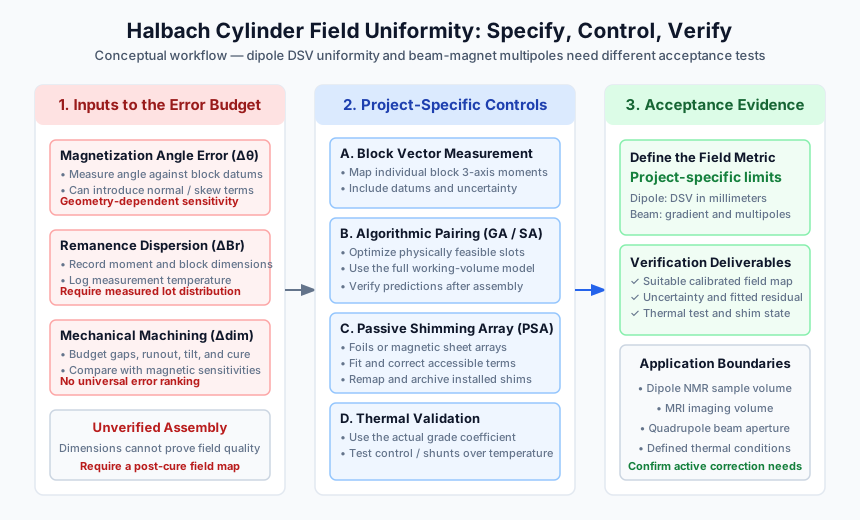
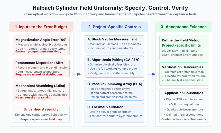Halbach Cylinder Field Uniformity: Error Budget and Mitigation Architecture Figure 1: A specification-to-verification workflow. This schematic illustrates error controls and required deliverables, not measured ppm improvements or a guaranteed shimming outcome.

1. Magnetization Vector Angular Deviation (Δθ)

During manufacture of anisotropic sintered NdFeB or SmCo, powder alignment establishes a preferred magnetization direction. The finished block's magnetic moment can deviate from its intended geometric axis. Require measured vector components relative to named block datums; a material grade alone does not establish an angular tolerance.

For a dipole segmented into N equal angular sectors, the nominal magnetization direction advances by 720°/N between adjacent sectors. Errors can introduce both normal and skew harmonics. Test proposed angular limits in the actual assembly model before selecting a purchase specification; an illustrative ±1° screening limit is not a universal acceptance rule.

2. Batch Remanence Spread (ΔBr)

Chemistry, processing, and temperature affect remanence, Br. Ask for the grade datasheet, lot-level measurements, and the distribution of finished-block magnetic moments rather than assuming a fixed percentage spread for all commercial magnets.

Unequal block moments perturb the intended bore field and can introduce gradients. Characterize moment magnitude together with volume: a larger block can have a larger magnetic moment without having a higher Br. Sorting must account for both geometry and magnetic measurements.

3. Mechanical and Glue-Line Tolerances (Δr, Δφ, Δz)

Mechanical errors contribute through several distinct mechanisms:

Radial runout and gap variation: Unequal bond lines change block positions and the magnetic fill factor. Calculate the field sensitivity using the actual segment geometry; a single inverse-distance law cannot describe all finite blocks.
Axial displacement and tilt: Segment misalignment changes axial gradients and end-field symmetry.
Adhesive cure: Shrinkage or fixture compliance can change the placement achieved during dry assembly.

Compare modeled perturbations in angle, moment, radial position, and tilt over the same working volume. Tighten the inputs that dominate that design's error budget, then verify the completed assembly magnetically.

4. Finite-Length End Effects

For an ideal infinitely long, continuously magnetized dipole cylinder with relative recoil permeability approximated as one:

B0 = Br × ln(Rout / Rin)

Finite length, segmentation, gaps, and material response change this result. End rings or changes in axial geometry may flatten the working region, but no single length-to-bore ratio guarantees a specified homogeneity.

Raich and Blümler (2004) describe a discrete bar-magnet dipole layout and compare simulation with Hall-probe measurements. Their results support evaluating the actual layout rather than treating the ideal-cylinder equation as an acceptance test.

Defining the Tolerance Budget: Spherical Harmonics and DSV

Before sending an RFQ to a magnet manufacturer, the engineering team must translate their application's functional requirements into rigorous mathematical specifications. A note such as "high field uniformity required" does not define a measurable acceptance criterion.

1. The Diameter of Spherical Volume (DSV)

Field uniformity is meaningless without a measurement region. Define the diameter of spherical volume (DSV) in millimeters, its center relative to assembly datums, and the sampling coordinates. A cylindrical NMR sample region can also be specified explicitly.

The usable region depends on bore size, length, segment layout, and shimming. A percentage of bore diameter is not a sufficient acceptance definition, and there is no universal 66% cutoff.

2. Quantifying Homogeneity: Peak-to-Peak vs. RMS

For a dipole NMR acceptance map, let Bi be the measured field magnitude at each point and B0 the agreed reference field, such as the nominal center field. Define the denominator explicitly.

Hpp (ppm) = (Bmax − Bmin) / B0 × 1,000,000 Hrms (ppm) = sqrt[sum wi × (Bi − B0)² / sum wi] / B0 × 1,000,000

Use equal weights only for an appropriate equal-volume sampling grid; a spherical-shell map needs stated weighting and reconstruction assumptions. Peak-to-peak and RMS limits are not interchangeable. Also agree the scan grid, interpolation method, temperature, measurement uncertainty, and handling of time drift during the scan.

Calculated RFQ example, not a measured assembly: Specify a 15 mm DSV and B0 = 1.000000 T. A hypothetical map spanning 0.999980–1.000020 T has Hpp = 40 ppm. If the agreed conservative acceptance rule is Hpp + U ≤ 50 ppm, an expanded uncertainty U = 5 ppm gives 45 ppm and passes; a 48 ppm map with the same U gives 53 ppm and does not pass. State the uncertainty coverage and decision rule in the purchase order.

Beam-optics boundary: A quadrupole's on-axis field is nominally zero, so dividing by B0 is inappropriate. Specify gradient in T/m, integrated gradient over the magnetic length, magnetic center, field angle, and allowed normal/skew multipoles at a named reference radius. A 3D DSV homogeneity number cannot replace these criteria.

3. Spherical Harmonic Decomposition

Set z along the bore axis and x along the nominal transverse dipole field. NMR acceptance concerns the magnitude |B|; a harmonic fit to the field component parallel to the main field approximates magnitude errors only when transverse perturbations are small.

A fitted basis may include linear terms X, Y, Z and second-order terms such as Z² − (X² + Y²)/2, X² − Y², XY, XZ, and YZ. Require the coordinate convention, coefficient units, reference radius, fitted order, and residual map. No single coefficient identifies one unique manufacturing defect.

For beam magnets, request a transverse normal/skew multipole expansion and its longitudinal integration convention instead. Check your supplier's magnetic inspection deliverables against the instrument's actual correction capabilities.

Pre-Assembly Mitigation: Combinatorial Algorithm Sorting (Genetic Algorithm Pairing)

One opportunity to improve Halbach cylinder field uniformity occurs before assembly, when block placement is still adjustable. This technique is known as Combinatorial Sorting or Algorithmic Block Pairing.

The Physics of Error Cancellation

The placement of measured blocks changes how their field errors superpose across the working region. Pairing can reduce selected harmonics without requiring every block to be perfect, but equal and opposite angle errors do not automatically cancel in geometrically opposite slots.

Optimize only physically interchangeable blocks, respecting each slot's required magnetization direction, allowed flips, mechanical datums, and assembly constraints. The objective must cover the full acceptance volume, not just the center point.

Measure block vectors → optimize feasible placements → archive numbered slot map → assemble and remap

The Sourcing Workflow for Block Pairing

Candidate pool: Agree whether spare blocks or a larger production lot are available for selection, and quote the material and measurement cost.
Individual vector characterization: Measure three-axis magnetic moment with a suitable calibrated coil/fluxmeter arrangement or equivalent scanner. Record moment magnitude, angular deviation from block datums, dimensions, and temperature.
Permutation solver: Evaluate feasible placements using a genetic algorithm, simulated annealing, or another validated optimizer coupled to a field model. Preserve the baseline and optimized predicted maps.
Assembly traceability: Archive block IDs, slot assignments, fixture references, and the final measured field map.

Economic boundary: Sorting adds metrology, modeling, and traceability work. It may reduce subsequent shimming effort, but neither a fixed ppm reduction nor a cost saving follows without geometry-specific predictions and assembled measurements.

Post-Assembly Passive Shimming Architectures

Sorting addresses known block variation, while post-assembly mapping captures residual placement and curing errors. The required combination of passive correction, active shim coils, and thermal control depends on the sample volume and NMR linewidth target.

Passive shimming uses permanent-magnet or ferromagnetic elements without continuous shim-coil current. It can reduce the active correction burden, but it is not mandatory for every instrument and cannot guarantee sub-ppm performance by itself.

1. Magnetic Sheet Arrays (MSAs) / Micro-Magnet Shimming

Wang et al. (2022) describe a passive Halbach shimming method based on magnetic sheet arrays. A practical implementation needs accessible shim locations, characterized shim responses, and a carrier compatible with the bore and RF probe.

Reserve the shim envelope before freezing the bore diameter.
Model or measure each candidate shim's field contribution.
Optimize placement against the measured residual map, including cross-coupling and clearance constraints.
Remap after installation and lock the final shim configuration in the assembly record.

2. Ferromagnetic Foil and Soft-Iron Shims

High-permeability foils or small soft-iron pieces can perturb local flux without requiring a permanent-magnet polarity pattern. Their response depends on shape, position, the background field, and the material's B–H curve.

Advantage: Simple shim pieces and potentially low material cost. Limitation: Saturation is not automatic, and hysteresis or magnetic history can affect repeatability. Characterize the installed response instead of assuming a constant dipole moment.

3. Rotatable Harmonic Corrector Rings

Jachmann et al. (2007) present permanent-magnet harmonic corrector rings for adjustable two-dimensional multipole shimming. This supports the correction concept, not a guaranteed 3D result for any Halbach cylinder.

Advantage: Mechanical adjustment can change correction harmonics without repeatedly replacing glued shims. Limitation: Rings consume space, require secure angular locking, and must be evaluated against the full volume and axial errors. Confirm which terms the proposed architecture can actually control.

Thermal Drift and Passive Flux Compensation

The temperature coefficient of remanence affects temporal stability as well as the apparent field map. Obtain the actual NdFeB or SmCo grade's coefficient, temperature interval, and irreversible-loss limits from its supplier datasheet.

For an assumed coefficient of −0.11%/°C and a 1.0 T field, a uniform 1°C rise would produce a first-order decrease of 1.1 mT, or 1,100 ppm. With a proton frequency coefficient of approximately 42.577 MHz/T, the corresponding frequency shift is about 46.8 kHz. These are calculated values for the stated assumptions, not measured drift data.

A uniform temperature change shifts the resonance frequency; temperature gradients can also change spatial uniformity. A frequency lock may track common drift but does not remove spatial gradients.

Mitigation Strategies

Thermal enclosure and control: Derive temperature stability from the allowed frequency drift and measured assembly coefficient. At the assumed −1,100 ppm/°C, even ±0.005°C corresponds to approximately ±5.5 ppm before compensation or frequency locking.
Thermomagnetic shunts: A suitable FeNi alloy can redistribute flux as its permeability changes with temperature. Specify the operating interval and setpoint, model its interaction with the field, and validate the residual drift and hysteresis in a chamber. Do not assume complete cancellation.
Recorded FAT conditions: Log magnet and probe temperature, equilibration time, scan duration, and reference-field readings. Remap after the agreed thermal cycle if repeatability is part of acceptance.

Sourcing Trade-Off Matrix: Homogeneity vs. Production Cost

Engineering and procurement should agree acceptance conditions before comparing quotes. This matrix is a sourcing decision aid, not empirical pricing or performance data. The only numerical acceptance example is the calculated 50 ppm case above; obtain project-specific feasibility, price, and lead time.

RFQ Goal	Acceptance Quantity	Working Region / Conditions	Manufacturing or Correction Choice	FAT Evidence to Request	Main Cost Driver
Center-field screening	Center field and field direction	Named center point at an agreed temperature	Dimensional control and basic magnetic inspection	Calibrated point measurement; cannot prove uniformity	Basic inspection scope
Dipole homogeneity	Peak-to-peak or RMS ppm with explicit B0	DSV in mm and a documented 3D grid	Vector characterization and feasible block sorting	Raw map, uncertainty, and acceptance calculation	Block metrology and selection inventory
Portable MRI	Field map compatible with the imaging/reconstruction specification	Actual imaging volume and thermal conditions	Geometry optimization, end correction, and optional shimming	3D magnitude/vector map and system-level imaging validation	Usable volume and integration effort
Benchtop NMR	Residual field map plus an agreed spectral linewidth test	Sample dimensions, nucleus, frequency, sample and temperature	Sorting, passive shims, and active correction as required	Before/after maps and linewidth with defined processing	Iterative mapping and shim access
Beam-optics quadrupole	Gradient, integrated gradient, normal/skew harmonics	Reference radius, magnetic length, and alignment datums	Multipole-specific block placement and correction	Rotating-coil or suitable longitudinal field-map report	Harmonic metrology and alignment
Temperature-stable field	Residual drift in ppm/°C and repeatability	Agreed setpoint, interval, dwell, and cycling history	Thermal control and/or qualified thermomagnetic shunts	Chamber log with field and temperature time series	Thermal validation and compensation development
High-temperature SmCo	Hot-field requirement and irreversible loss after cooling	Agreed operating/soak temperature and environment	Qualified grade, housing, adhesive, and retention	Hot/cold maps and thermal-cycle loss report	Material, mechanical retention, and environmental testing
Miniature bore	Uniformity or gradient appropriate to the instrument	Explicit usable sample region and probe clearance	Small-segment fixtures and accessible shim carrier	Probe active area, positioning uncertainty, and mapped coverage	Probe access and assembly fixturing

The Procurement & RFQ Engineering Checklist

When releasing an RFQ package or manufacturing drawing, use this checklist to turn field quality into a reviewable acceptance plan:

1. Define the field type and region: For a dipole, state the DSV in mm and its center relative to assembly datums. For a quadrupole, state reference radius, gradient, integrated gradient, and allowed harmonics.
2. Fix the calculation and decision rule: Define B0, peak-to-peak or weighted RMS, the limit, measurement uncertainty, and any guard band. Preserve the raw data used for acceptance.
3. Agree block-vector limits: Specify moment magnitude and angle relative to named datums, with a measurement method and uncertainty. Derive angular tolerances from sensitivity analysis rather than adopting a universal ±1° rule.
4. Require placement traceability: If sorting is included, request the feasible-slot constraints, predicted improvement, numbered block assignment, and final measured result. An algorithm name alone is not evidence of performance.
5. Assign shimming responsibility: Identify who supplies the carrier, installs shims, remaps the assembly, and owns final acceptance. State the bore clearance remaining for the RF probe or beam tube.
6. Define harmonic deliverables: Require the coordinate basis, reference radius, units, fitted order, and residual map; distinguish spherical dipole fits from integrated beam multipoles.
7. Record temperature and stability: Agree setpoint, equilibration, drift during mapping, thermal cycling, and any frequency-lock or active-shim state.
8. Qualify the measurement system: Specify scan coverage and spacing from the expected spatial errors, probe size, calibration, positional uncertainty, and overall uncertainty. Use an NMR field/linewidth method where the required precision exceeds Hall-probe capability.

Frequently Asked Questions (FAQ)

Q1: Why not just use active shim coils instead of passive sorting and shimming?

A: Active coils can provide final correction, but their range, power dissipation, space, and supply stability are limited. As a calculated scale example, 3,000 ppm of a 1 T field is 3 mT, whereas 20 ppm is 20 µT. Actual current and heat depend on coil sensitivity and resistance. Reducing the residual error can reduce the active burden; active coils still generate heat when energized.

Q2: How many segments should we choose: 8, 12, 16, or 24?

A: Compare the same bore, outer diameter, length, gaps, and working volume. For ideal equal angular sectors in an infinite dipole cylinder, the segmentation field factor is sin(2π/N)/(2π/N): approximately 90.0% for 8, 95.5% for 12, 97.4% for 16, and 98.9% for 24 segments.

These calculated factors describe ideal field strength, not delivered homogeneity. More segments add assembly interfaces and inspection work while changing discretization harmonics. Use the modeled field map and quoted process capability to decide; a discrete bar-magnet layout needs its own model.

Q3: Can wire-EDM create a Halbach cylinder from a conventional uniformly oriented sintered ring?

A: Cutting changes geometry, not the material's magnetic easy-axis distribution. A conventional uniformly oriented sintered ring does not acquire a rotating Halbach magnetization merely by machining or by a stronger magnetizing pulse. Conventional sintered constructions use separately oriented segments. Specialized oriented or bonded-magnet processes are different manufacturing routes and need their own qualification.

Q4: How does adhesive shrinkage affect homogeneity during curing?

A: Cure shrinkage and fixture compliance can shift or tilt segments under magnetic forces. The resulting ppm error depends on geometry and cannot be inferred from a universal micrometer-to-ppm conversion. Agree bond-line thickness, adhesive compatibility, cure schedule, fixture constraint, and a post-cure magnetic map. Compare pre- and post-cure data when qualifying the process.

Q5: What is the difference between dipole and quadrupole field acceptance?

A: With z along the bore axis, a dipole has a nominally uniform transverse field, for example Bx ≈ B0, and is commonly used for NMR/MRI. An ideal quadrupole has zero field at its center and a linear transverse gradient; one orientation is Bx = G·y and By = G·x. It focuses one transverse beam plane while defocusing the other.

Specify dipole uniformity over a sample volume. Specify quadrupole gradient, magnetic center, alignment, integrated strength, and higher multipoles over the beam aperture. Do not normalize quadrupole error by the zero center field.

Conclusion: Engineering Your Supply Chain for Magnetic Precision

A precision Halbach cylinder needs dimensional control and magnetic acceptance that refer to the same working region, coordinate system, temperature, and correction state. Measured block vectors and feasible placement optimization address pre-assembly variation; post-cure mapping determines whether passive or active correction is needed.

Before comparing suppliers, ask which measurements are included, what uncertainty they can support, who owns shimming, and what happens if the delivered field fails the agreed limit. These decisions are more useful than a generic claim of “high homogeneity.”

Partner with Halbach Magnet on Your Precision Assembly

Explore the Halbach Cylinders Product Family, review the Precision Quality Control & Metrology Capabilities, or discuss the modeling scope through Custom Engineering Services.

Contact our engineering and procurement team with bore and envelope dimensions, field type, working volume or reference radius, target field quality, operating temperature, and quantity. Ask the project team to confirm the available block measurements, sorting, shimming, FAT deliverables, and confidentiality arrangements during the quotation review.

Sources & References

H. Raich and P. Blümler, Design and construction of a dipolar Halbach array with a homogeneous field from identical bar magnets: NMR Mandhalas, Concepts in Magnetic Resonance Part B: Magnetic Resonance Engineering, Vol. 23B, No. 1, pp. 16–25 (2004). DOI: https://doi.org/10.1002/cmr.b.20018.
R. C. Jachmann, D. R. Trease, L.-S. Bouchard, D. Sakellariou, R. W. Martin, R. D. Schlueter, T. F. Budinger, and A. Pines, Multipole shimming of permanent magnets using harmonic corrector rings, Review of Scientific Instruments 78, 035115 (2007). DOI: https://doi.org/10.1063/1.2713438.
Ya Wang, Yajie Xu, Feng Wang, Junhao Zhang, Bowen Peng, Peng Yu, Yingcong Yu, and Xiaodong Yang, A passive shimming method for Halbach magnet based on magnetic sheet arrays, Journal of Magnetic Resonance 339, 107210 (2022). DOI: https://doi.org/10.1016/j.jmr.2022.107210.

All Posts

Author

Kenneth Adler - Principal Magnetic Circuit Engineer